Author: Henry Rzepa

  • An unusually small (doubly) aromatic molecule: C4.

    When you talk π-aromaticity, benzene is the first molecule that springs to mind. But there are smaller molecules that can carry this property; cyclopropenylidene (five atoms) is the smallest in terms of atom count I could think of until now, apart that is from H3+ which is the smallest possible molecule that carries σ-aromaticity. So here I have found what I think is an even smaller aromatic molecule containing only four carbon atoms. And it is not only π-aromatic but σ-aromatic.

    Let me go through the analysis (using a CCSD(T)/Def2-TZVPPD calculation, DOI: 10.14469/hpc/10226).

    1. Four carbons contain 16 valence electrons for bonding.
    2. Eight of these are conventional, forming four C-C single bonds around the 4-ring.
    3. Eight are left over, and these partition into a set of six and a set of two.
    4. The set of two are in p-π atomic orbitals and form a 4n+2 (n=0) aromatic system
    5. The set of six are in σ-sp AOs and form a 4n+2 (n=1) aromatic system.
    6. The three σ-MOs all contribute to the central C-C bond, particularly σ3 and σ2 in different ways.
    7. σ2 also reminds of [1.1.1]-propellane, where the two σ-electrons are in effect external to the central C-C bond, but spin coupled to form what might be called a σ exo-bond. There is also similarity to the exo bond in C2.
    8. The dissociation energy of the central bond can be estimated at 28 kcal/mol from the triplet state energy.
    Bonding MOs for C4.
    Click image to load 3D model
    π1
    σ3 σ2
    σ1

    So this little molecule carries a lot of diversity in its chemical bonding; an ideal candidate perhaps for a tutorial in bonding theory of organic molecules?


    The post has DOI: 10.14469/hpc/10252

  • Raw data: the evolution of FAIR data and crystallography.

    Scientific data in chemistry has come a long way in the last few decades. Originally entangled into scientific articles in the form of tables of numbers or diagrams, it was (partially) disentangled into supporting information when journals became electronic in the late 1990s.[cite]10.1021/acs.orglett.5b01700[/cite] The next phase was the introduction of data repositories in the early naughties. Now associated with innovative commercial companies such as Figshare and later the non-commercial Zenodo, such repositories have also spread to institutional form such as eg the earlier SPECTRa project of 2006[cite]10.1021/ci7004737[/cite] and still evolving.[cite]10.1186/s13321-017-0190-6[/cite] Perhaps the best known, and certainly one of the oldest examples of curated structural data in chemistry is the CCDC (Cambridge crystallographic data centre) CSD (Cambridge structural database) which has been operating for more than 55 years now, even before the online era! Curation here is the important context, since there you will find crystal diffraction data which has been refined into a structural model, firstly by the authors reporting the structure and then by CSD who amongst other operations, validate the associated data using a utility called CheckCIF.[cite]10.1107/s090744490804362x[/cite] What perhaps is not realised by most users of this data source is that the original or “raw” data, as obtained from a X-ray diffractometer and which the CSD data is derived from, is not actually available from the CSD. This primary form of crystallographic data is the topic of this post.

    Most chemical data now emerges from an instrument, where it is already partially processed internally before being offered. Such raw/primary data is perhaps best known in the form of NMR information, where it is offered by the instrument in the form of an FID or free induction decay. Its transformation from this form into what all chemists know as a spectrum requires further software processing, and including other operations such as peak integration. It is this processed spectrum that had traditionally been offered as part of a scientific article (often only in visual, or peak listed form) and rarely has the FID form been made available to anyone interested. It is important to state that the transformation to spectrum also incurrs significant loss of data. An interesting project led by the editors of two organic chemistry journals[cite]10.1021/acs.joc.0c00248[/cite],[cite]10.1021/acs.orglett.0c00383[/cite] had the aim of encouraging the submission of FAIR data to the journal, although in fact the project actually concentrated on the submission of raw NMR data. As it turned out, only a very small proportion of all the submissions to these journals over the period of a year actually provided such data (~113 datasets) in the form of ZIP archives and containing anywhere between one and ~100 actual sets of raw NMR data per archive. One should make the point that raw data is not necessarily FAIR data. The latter requires rich metadata describing the data to become findable, accessible, interoperable and reusable (FAIR), and such metadata was not actually generated as part of this publisher project. 

    Here I will take a closer look at potentially FAIR raw data in the area of crystallography. This project is perhaps less well known than the previous one,[cite]10.1021/acs.joc.0c00248[/cite],[cite]10.1021/acs.orglett.0c00383[/cite] hence the present post strives to make it better known. As with NMR, a useful starting point is to describe the various stages in the lifecycle of crystal data.

    1. A crystal is mounted in the diffractometer and x-ray diffraction images are recorded. These are considered the raw data, and as with most instruments, their form is determined both by the instrument itself and the software used to start the refinement process into a molecular structure.
    2. This refinement then assigns a space group to the data and derives so-called structure factors or hkl data. This data can now be captured in a much more standard form known as a CIF (crystallographic information file) and is nowadays the format that is deposited with CSD.
    3. A reduced form of the CIF file, containing a sub-set of the information but lacking the hkl data is much the more common, and was the form originally sent to CSD until a few years ago.
    4. Very often an image of the resulting model for the molecular structure is also included. Whilst it is based on the data in the CIF file, it does not contain reusable data as such and is considered as being made available only for human use and perception.

    It is form 1 that is missing from the CSD datasets. Because it can be quite large (~0.5-9 Gbyte), the current recommendation is that it is not stored on the CSD but on local data repositories. So now we see a need to establish if possible bidirectional links between type 1 and types 2-4 and to identify what characteristics of FAIR each has. Primarily, the F (findable) of FAIR will be explored here. This is done by illustrating some searches for this data, based on the metadata registered for it with DataCite.

    1. https://commons.datacite.org/?query=relatedIdentifiers.relatedIdentifier:10.5517*  (157 works)
      This simple search identifies any entry in any repository which cites in its metadata record the DOI for an entry in CSD, taking the form 10.5517* which is common to all entries.
    2. ?query=relatedIdentifiers.relatedIdentifier:*10.5517*+AND+(media.media_type:chemical/x-cif+OR+media.media_type:application/x-7z-compressed+OR+media.media_type:application/gzip+OR+media.media_type:application/zip) (9 works).
      This also specifies that search 5 is further constrained by requiring one of four media types to ALSO be present in the repository metadata record. These types are standard compressed archives which the raw crystal data is likely to be stored as, along with a CIF entry that is clearly associated with crystal structure data. The Boolean OR indicates that any one of them can be present! One can now be a little more certain that these entries contain crystal structure data. That we cannot be absolutely certain is clearly a current deficiency of the metadata present for the entries! 
    3. ?query=identifier:*10.5517*+AND+(relatedIdentifiers.relatedIdentifier:*10.14469*) (7 works)
      Eight works from search 6 originate from a repository with the prefix 10.14469* and so now one can reverse the direction and ask how many are referenced in the metadata for each published item in the CSD? Around 945,473 entries in the CSD currently have a persistent DOI identifier associated with them, all starting with 10.5517* and so now one can search for how many of these also reference a related identifier at 10.14469*  Seven of them show up there.
    4. Also in the CSD metadata records is an item with the attribute relationType=”IsDerivedFrom” carrying the meaning that the CSD data is itself derived from (raw) data held elsewhere. This information is captured during the deposition process with CCDC as per below.

      https://commons.datacite.org/?query=identifier:*10.5517*+AND+(relatedIdentifiers.relationType:IsSourceOf+OR+relatedIdentifiers.relationType:IsDerivedFrom)  (7 works)
      This constrains to datasets at CSD that are associated with additional raw data by IsDerivedFrom or IsSourceOf relationships. CCDC tell me the true number is around 65 so the origins of this mismatch need to be identified.

    So projects aiming to capture data from chemical instrumentation are just starting to reveal the potential of this modern system for storing data in two or more locations and reconciling various forms of this data, from raw form to derived or processed data. The interested user can then use whichever form is most relevant to their needs, and having found one form can then trace back to the other form(s). We might anticipate many developments in this area in the near future. 


    One has to expand the archive to find out how many actual raw datasets are inside, rather than knowing beforehand how many datasets are contained there, or anything else about their properties. The publication process is described here for one repository at DOI: 10.14469/hpc/10178 From the DataCite schema; <relatedIdentifier relationType="IsDerivedFrom">... </relatedIdentifier> IsDerivedFrom should be used for a resource that is a derivative of an original resource. In this example, the dataset is derived from a larger dataset and data values have been manipulated from their original state. <relatedIdentifier relationType="IsSourceOf">... </relatedIdentifier> IsSourceOf is the original resource from which a derivative resource was created. In this example, this is the original dataset without value manipulation.


    This post has DOI: 10.14469/hpc/10177


  • Chasing ever higher bond orders; the strange case of beryllium.

    Ever since the concept of a shared two-electron bond was conjured by Gilbert N. Lewis in 1916,[cite]10.1021/ja02261a002[/cite] chemists have been fascinated by the related concept of a bond order (the number of such bonds that two atoms can participate in, however a bond is defined) and pushing it ever higher for pairs of like-atoms. Lewis first showed in 1916[cite]10.1021/ja02261a002[/cite] how two carbon atoms could share two, four or six electrons to achieve a bond order of up to three. It took quite a few decades for this to be extended to four for carbon (and nitrogen) and that only with some measure of controversy and dispute (for one recent brief summary, see[cite]10.1039/D1CP02056K[/cite]).

    For the transition elements over the last forty years or so, bond orders of four, five and even six between like atom pairs have been mooted and many characterised.[cite]10.1002/anie.201504414[/cite] Moving to the left of the transition elements in the periodic table, this hunt has looked at elements such as beryllium. Eleven years back, I explored here how a Be=Be double bond could be formed, strangely enough as an electronically excited state of the dispersion-bound weak Be2 dimer.[cite]10.1139/v96-111[/cite] This species had a calculated Be-Be distance of 1.78Å, resulting from double excitation from the 2s σ*-antibonding orbital into the degenerate π-bonding orbital above it, giving four electrons in bonding valence orbitals. In 2019, three articles appeared which showed how this bond order might be extended to the lofty heights of three as in Be≡Be[cite]10.1002/cphc.201900051[/cite],[cite]10.1039/c9dt03321a[/cite],[cite]10.1016/j.cplett.2019.06.023[/cite] for (hypothetical) molecules in their ground electronic state. Here I discuss one example from these articles and compare it to the excited state observations made previously.

    A useful starting point is the standard molecular orbital diagram for Be2, illustrating why the ground state singlet actually has a bond order of zero.

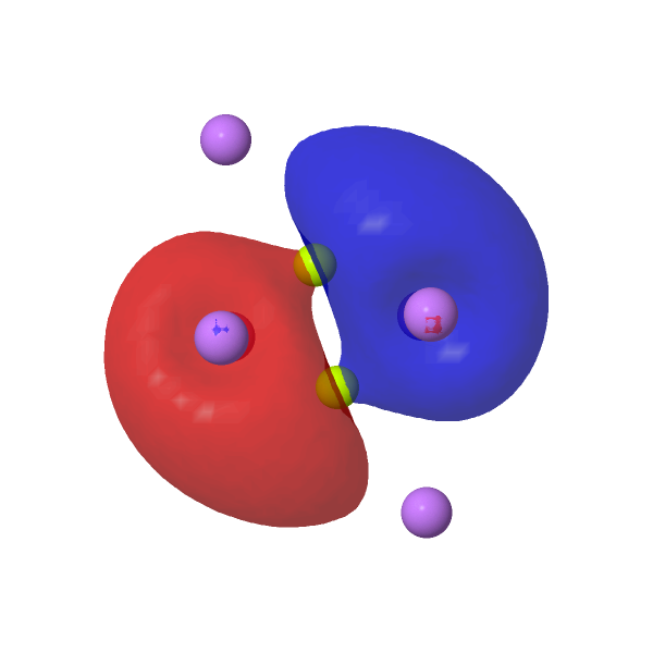
    The three 2019 suggestions[cite]10.1002/cphc.201900051[/cite],[cite]10.1039/c9dt03321a[/cite],[cite]10.1016/j.cplett.2019.06.023[/cite] modified this to surround the Be2 core with e.g. six Li atoms, resulting in a stable singlet species with a Be-Be distance (calculated at e.g. the CCSD/Def2-TZVP level) of 1.99Å and exhibiting C2h symmetry. The role of the Li is to polarise and repopulate Be orbitals by delocalization of e.g. a 2c-2e bond in Be2 dimer into a 6c-2e bond in Be2Li6. The reported calculations (as successfully replicated here, FAIR DOI: 10.14469/hpc/10106) show the resulting molecular orbitals for Be2Li6 comprise an (accidentally) degenerate π-pair and a higher energy weak σ-orbital, together forming the proposed triple bond. This of course inverts the normal ordering of such bonds, for which the σ-orbital is lower in energy (more stable) than π-bonds. The form of the σ-orbital also reminds to some extent of the fourth σ-bond in C⩸C.

    MOs for Be2Li6

    HOMO, σ orbital

    -0.158au

    HOMO-1, π-pair,

    -0.175au

    HOMO-2, π-pair

    -0.176au

    Because the static 2D projections shown in the articles cited above do not always make for easy interpretation, if you click on the orbital thumbnails, you will get dynamic 3D isosurfaces to rotate and inspect. These were generated using the tool at https://www.ch.ic.ac.uk/rzepa/cub2jvxl/

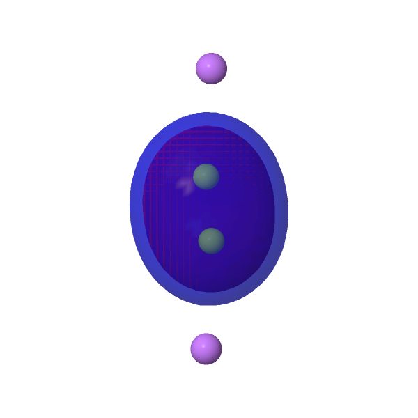
    The two lower energy 2s σ-orbitals, which taken together do not apparently contribute to the overall bond order in Be2Li6, are shown below.

    Lower energy MOs for Be2Li6
    σ -0.235au σ-0.496au

    ELF (electron localisation function) integrations for Be2Li6 show each beryllium has two basins in the Be-Be region of about 2.5e each (red arrows) typical of triple bonds and two terminal Li-Be basins of 2.3e.

    One aspect arising from my earlier post on the excited state Be=Be double bond relates to the reported calculated Be-Be bond length of 1.99Å and ν 718 cm-1 for ground state Be2Li6. To quote one article[cite]10.1002/cphc.201900051[/cite], “the Be≡Be triple bond in Li6Be2 may also be considered as another example of an ultraweak but ultrashort triple bond.” I had noted earlier that the electronically excited state of the Be2 dimer has a computed bond length of 1.78Å and ν 917 cm-1 for a double bond order, this being significantly shorter than the suggested ultrashort triple bond. We learn from this that the relationship between a bond order and a bond length may not always be linear. In other words, a longer bond may in fact have a higher bond order than a shorter bond between the same two atoms. The same was true as it happens with C⩸C; the mooted quadruple bond had a longer bond length than the triple bond in HC≡CH. That observation was controversial at the time; I suspect a similar phenomenon for Be has become less controversial.

    To go back to the Be=Be dimer which started things off and that excited state with one electron in each of the degenerate π-orbitals (actually a triplet state). What would happen if two electrons were to be added, making an excited state of Be22-? Yes indeed, this species (CCSD/Def2-TZVPPD) has a calculated bond length of 1.885Å and ν 766 cm-1. If this di-anion is stabilised with a continuum water field (a milder version of surrounding the dimer with Li atoms), the Be-Be length contracts to 1.74Å, the Be-Be stretch increases to 949 cm-1 and the σ-orbital becomes more stable than the π-orbitals. At the higher CCSD(T)/Def2-TZVPPD/SCRF=water level, the bond length still has the ultrashort value of 1.761Å, which might be assumed as the natural value for Be≡Be, a classical triple bond. From that perspective, the “ultraweak but ultrashort triple bond” predicted for Be2Li6 actually emerges as a relatively long triple bond!

    Our final exploration is to add two lithium atoms to Be2 to form the neutral LiBe≡BeLi. This was done in stages (see FAIR DOI 10.14469/hpc/10106), starting with a linear arrangement of atoms which revealed two negative force constants, a C2h shape with one negative force constant and ending with a C2 (chiral!) geometry with no negative force constants. This has a Be≡Be length of 1.705Å (ωB97XD/Def2-TZVPPD/SCRF=water), ν 1129 cm-1, a Wiberg bond index of 2.98 and a Li-Be bond index of 0.0065, indicating an entirely ionic lithium and again a central Be22- unit. As an excited state, it is 49.8 kcal/mol higher than the ground state of Be2Li2.

    NBOs for LiBe≡BeLi

    HOMO, π-pair,

    -0.175au

    HOMO, π-pair

    -0.176au

    HOMO-2, σ orbital

    -0.158au

    So to conclude, we have seen two different motifs for constructing a model of a Be≡Be triple bond, one recently reported in the literature for a ground state species with six lithium atoms surrounding the Be2 dimer and a simpler one with just two lithiums exhibiting a much shorter Be≡Be bond but which requires electronic excitation to achieve. So these two motifs are not equivalent. But hopefully this exercise shows how playing around with atoms and electrons can achieve very unusual bonding states and elevated bond orders from which one can learn a lot, although with the caveat that one does not always produce molecules capable of facile synthesis!


    On a slightly different theme, Cs can be shown to sustain three bonds, albeit all to different atoms. See DOI: 10.6084/m9.figshare.861030 Li≡Li4- can also be calculated as the tetra-anion showing almost identical properties to Be≡Be2- with a Li≡Li triple bond distance of 2.11Å. See DOI: 10.14469/hpc/10122. Replication was necessary because the appropriate wavefunction files for analysis were not included in the supporting information. Only the coordinates were available for interoperation, and due to a quirk in the way Adobe Acrobat works, even those could not be easily transferred by a simple copy/paste operation to create a job input file. See e.g. here or DOI: 10.14469/hpc/10043 for more discussion. All the wavefunction files for this replication are available at the FAIR DOI noted above. The Be-Be distance in catena(dimethylberyllium), a polymer comprising two bridging Me units connecting Be atoms, is only slightly longer at 2.09Å[cite]10.1107/S0365110X51001100[/cite] This fascinating transannular Be-Be interaction is one to be explored elsewhere.


    The post has DOI: 10.14469/hpc/10125


  • Data base or Data repository? – A brief and very selective history of data management in chemistry.

    Way back in the late 1980s or so, research groups in chemistry started to replace the filing of their paper-based research data by storing it in an easily retrievable digital form. This required a computer database and initially these were accessible only on specific dedicated computers in the laboratory. These gradually changed from the 1990s onwards into being accessible online, so that more than one person could use them in different locations. At least where I worked, the infrastructures to set up such databases were mostly not then available as part of the standard research provisions and so had to be installed and maintained by the group itself. The database software took many different forms and it was not uncommon for each group in a department to come up with a different solution that suited its needs best. The result was a proliferation of largely non-interoperable solutions which did not communicate with each other. Each database had to be searched locally and there could be ten or more such resources in a department. The knowledge of how the system operated also often resided in just one person, which tended to evaporate when this guru left the group.

    After the millennium, two newcomers started to appear, one being called an ELN (electronic laboratory notebook) and the second a data repository. The first was a heavily customised database containing research data as obtained from instruments, computers, images/video, chemical structure drawings etc. ELNs, even to this day, have limitations of interoperability with other ELNs and the contents of an ELN are often closed, requiring authentication credentials to access. The data repository also started to appear in chemistry around this period. Even in its early incarnations, it could be associated with an ELN “front end” as part of the data pipeline; an early example of this coupling is described here.[cite]10.1021/ci500302p[/cite] Another key phrase that became associated with repositories starting around 2014 was the concept of FAIR, including ideas such as the Findability (discoverability) and Interoperablity of data, a theme often explored and illustrated on this blog.

    These last seventeen years has seen organisations such as funding agencies and publishers increasingly mandating the use of such data management methods, using either a repository on its own or a combination of an ELN and repository as routine operations in research activity and publication processes. The close coupling of an ELN and repository is still however uncommon. 

    A colleague recently alerted me to a computational chemistry repository first launched in 2014; www.iochem-bd.org  Reading the about text, I found these statements;

    • Chem-BD is a digital repository aimed to manage and store Computational Chemistry files.
    • Goals: Build a distributed database of computational chemistry results: reduce size and increase value.
    • Set a common data standard among all quantum chemistry legacy formats (XML – CML[cite]10.1021/ci990052b[/cite])

    So this is both a database and a data repository, as well as espousing a commendable common data standard![cite]10.1021/ci990052b[/cite] I decided to explore the first two aspects here using this resource as an example.

    • Whilst the absolute distinction between the two types can be blurry, the crucial difference between the two is that a database functions on curation via a structured index of the data, whilst a repository aspires to having FAIR attributes primarily through its metadata as exposed by registration (metadata is data describing the data).
    • A database holds this data index locally and the Findability of the data is associated purely with the functionality of  the database. The data structures are defined by a database schema, describing in detail all the terms indexed (a key and its value) and searched using the values of these key pairs. This schema is unlikely to be exactly the same as e.g. databases on related topics, largely because the database is self-contained and self-consistent.
    • A data repository also uses a schema (DOI: 10.14454/3w3z-sa82 and[cite]10.1002/leap.1429[/cite]) to express the key pairs, but this time it is expressed as metadata. Now, this metadata is registered externally to the repository using a registration agency.[cite]10.1002/leap.1429[/cite] The metadata for each deposited object is assigned a persistent identifier known as a DOI. Although it might be indexed and searchable locally, it must be capable of also being searched in aggregated/federated form using services provided by registration or other agencies. This independence of metadata is part of those FAIR criteria.
    • Whereas a database can be very finely grained in order to describe individual properties of an object, repository metadata tends to be more coarsely grained to describe the object as a whole, to place it in context and to impart provenance.
    • Both databases and repositories can have what is called an API (application programmer interface) to allow machine access (the A of FAIR) to the contents. Accessing the former would normally require bespoke code to be written and possibly authentication credentials, whereas information to access to repository held data is provided via the registered metadata (which does not normally require credentials). Access to the repository may also require code, but if the metadata is carefully standardised by adherence to the schema, the code can be made more general than that required for a database.
    • A typical entry in the www.iochem-bd.org repository has a DOI of 10.19061/iochem-bd-4-36
    • This DOI is registered with the CrossRef agency, one normally used for registering journal articles, rather than DataCite which is used for registering data and other research objects. The metadata for this DOI can be viewed using the resolution service https://api.crossref.org/works/10.19061/iochem-bd-4-36/transform/application/vnd.crossref.unixsd+xml and shows that it largely contains the bibliographic information typical of a journal article. So in this sense it is certainly a repository, but using a metadata schema that is more frequently used for journal articles than for data sets.
    • The CrossRef metadata record also has an item <resource>https://www.iochem-bd.org/handle/10/235025</resource> which points to the so-called landing page for that item, but information about the properties of the actual data itself must be instead obtained directly from the repository. 
    • Because the metadata describing the data is only held at this repository and not elsewhere (a local metadata record), it can only be queried locally and the query cannot be upon aggregated metadata  provided by the registration agency. A machine query would have to be constructed by coding a suitable request using the API provided for the database aspect of this repository. 

    This example has served to highlight just a few of the often quite subtle distinctions between eg a database and a data repository and that some examples can indeed be both.  It also highlights that repositories can have the attributes of  FAIR, which in themselves are driven by asking “what could a machine do to obtain data?” rather than what could a human achieve by browsing. So another question that arises when evaluating the characteristics of a repository is whether each item held there has a FAIR-enabling metadata record describing the data, a record which is registered in a manner that can be aggregated and hence used to find and access content across multiple independent repositories.


    This post has DOI 10.14469/hpc/10043


    Indeed in that era, few online/Internet infrastructures were available as part of departmental resources. See also here.  In this last regard, I note a workshop devoted largely to such interoperability and machine access in chemistry coming up soon; https://www.cecam.org/workshop-details/1165 The CrossRef schema is not referenced using an assigned DOI: data.crossref.org/reports/help/schema_doc/5.3.1/.An example can be seen at doi: 10.14469/hpc/10059 Here, invoking a hyperlink based purely on the data DOI and the data media type required in turn calls code (Javascript) which retrieves the metadata held for that DOI and parses it to identify whether it indicates the presence of a file manifest. If it does, it identifies the type of manifest (ORE in this case) and the media types the manifest points to and finally uses that manifest to then retrieve data filtered by media type and pipes it into a visualiser (JSmol). In this case the endpoint is visualisation, but it could also be eg piped into an AI/ML program for analysis. In this case only one instance of data is machine retrieved, but in principle it could be a multitude of data files obtained from a multitude of different locations and based on a multitude of criteria as filtered by suitable searches of registered metadata.[cite]10.1002/mrc.5186[/cite]


  • Quantum chemistry interoperability (library): another step towards FAIR data.

    To be FAIR, data has to be not only Findable and Accessible, but straightforwardly Interoperable. One of the best examples of interoperability in chemistry comes from the domain of quantum chemistry. This strives to describe a molecule by its electron density distribution, from which many interesting properties can then be computed. The process is split into two parts:

    1. Computation of the wavefunction. This can be very very compute intensive process, which can take quite a few days even using 64 or more processors in parallel and requires highly specialised programs to achieve this.
    2. Analysis of the wavefunction. The range of properties that can be computed is impressively large, but again this requires specialised algorithms and programs.

    So one can see that the need to Interoperate wavefunction data computed during process 1 into analysis in process 2 is crucial. This is normally achieved using intermediate data files, and clearly the semantics of the data in these files must be perfectly communicated between the two processes.

    With this introduction over, my attention was drawn to a recent post on the CCL (Computational Chemistry List, http://www.ccl.net), a veritable resource that has been running for many decades and where many aspects of computational chemistry are discussed. One recent such relates to quantum chemistry interoperability; http://www.ccl.net/cgi-bin/ccl/day-index.cgi?2021+12+30 where many interesting points were made. I highlight just two here (but urge you to read the entire thread).

    1. The first, by Mike Frisch (http://www.ccl.net/cgi-bin/ccl/message-new?2021+12+30+003) introduces two interoperability formats (the binary array file format) along with a library of routines in both Fortran and Python which facilitate interoperability between wavefunction calculating and the post-processing analysis programs. The advantages of this include “Like the fchk file, this is a self-defining file, but it is binary so that full precision can be retained and reading/writing the file is much faster” and is described at https://gaussian.com/interfacing/ Output in this format is controlled by the keyword Output=MatrixElement or use of environment variables. As a long time user of an older interoperability mechanism, the so-called WFN and WFX formats for use with programs such as AIMALL and MultiWFN, I have often set this keyword to eg Output=wfn and when generated, such files are routinely included in our FAIR data publications which are often mentioned both in this blog and in the journal articles we write. If you read the post by Mike, you will understand both the deficiencies of these earlier formats and how the binary array file is an important advance. 
      • I make one “user interface plea” here in the hope that Gaussian might be able to do something about it. By default, the output key word is not set and so no wavefunction data is produced other than a binary .CHK file. This in turn requires an extra step to convert it into the interoperable non-binary .FCHK file. When needing a WFN file, very often I forget to set the output keyword flag to a value and have to re-run the program to obtain it. So my plea is to consider setting the program defaults to write out some form of the binary array file when the job completes. There are additional flags that can be set for specialised applications, but assuming a default option would be practical, it would be good to have.
    2. The second email is a response to Mike’s post by Tian Lu  who is well known for his amazing “swiss army knife” program MultWFN, which can compute a large variety of molecular properties using wavefunction files. He had in fact proposed his own interoperability format to eliminate many of the recognised issues with the older WFN, FCHK and WFX formats and which is called MWFN (documented here[cite]10.26434/chemrxiv-2021-lt04f-v5[/cite]). Currently this particular format is not yet widely supported by wavefunction-computing programs such as e.g. Gaussian, but perhaps Output=mwfn will come one day!
    3. This is a later email describing the Trexio Project (https://trex-coe.github.io/trexio/ and specifically https://trex-coe.github.io/trexio/trex.html) in which a metadata group is specifically identified because “we need to give the possibility to the users to store some metadata inside the files.” In fact, metadata is also useful for registration with metadata agencies.

    This increasing discussion of Interoperability in Quantum Chemistry has to be warmly welcomed. It directly feeds into FAIR data and may even set a trend for other areas of chemistry, such as e.g. NMR spectroscopy!


    I have now learnt that inserting one of the environment variables below as per

    export GAUSS_OMDEF=fortranbinaryarray.faf
    or
    export GAUSS_ORDEF=rawbinaryarray.baf

    into job scripts will achieve this (proposed media types chemical/x-rawbinaryarray  .baf and chemical/x-fortranwbinaryarray  .faf).

    Currently doing both at the same time is not supported (G16 C C.01), so the second file can be generated from a .chk file using the post-processing commands appended to the job script:

    formchk -raw mychk.chk rawbinaryarray.baf
    or
    formchk -mat mychk.chk fortranbinaryarray.faf


    This post has DOI: 10.14469/hpc/10043


  • Molecule of the year 2021: Infinitene.

    The annual “molecule of the year” results for 2021 are now available … and the winner is Infinitene.[cite]10.33774/chemrxiv-2021-pcwcc[/cite],[cite]10.1021/jacs.1c10807[/cite] This is a benzocirculene in the form of a figure eight loop (the infinity symbol), a shape which is also called a lemniscate [cite]10.1021/jo801022b[/cite] after the mathematical (2D) function due to Bernoulli. The most common class of molecule which exhibits this (well known) motif are hexaphyrins (hexaporphyrins; porphyrin is a tetraphyrin)[cite]10.1039/b502327k[/cite],[cite]10.1021/ol0521937[/cite],[cite]10.1002/chem.200600158[/cite], many of which exhibit lemniscular topology as determined from a crystal structure. Straightforward annulenes have also been noted to display this[cite]10.1107/S1600536811048604[/cite] (as first suggested here for a [14]annulene[cite]10.1021/ol0518333[/cite]) and other molecules show higher-order Möbius forms such as trefoil knots.[cite]10.1038/NCHEM.1955[/cite],[cite]10.1039/D0CC04190D[/cite] This new example uses twelve benzo groups instead of six porphyrin units to construct the lemniscate. So the motif is not new, but this is the first time it has been constructed purely from benzene rings.

    The molecule has D2 chiral symmetry and is shown below (click on the image for the 3D model obtained from the crystal structure).

    The authors suggest that the aromaticity in a D2-symmetric [12]-circulene is confined to six “Clar” rings each of six electrons, and is not delocalised around the entire molecule. For a molecule with this topology (defined by a linking number, Lk = 2π[cite]10.1016/j.comptc.2014.09.028[/cite]) the entire system would be defined as aromatic (delocalised) for 4n+2 electrons and antiaromatic for 4n electrons around a continuous annulene loop. In this example outer annulene circuits of either 34 or 38 carbons can be constructed which retain D2-symmetry and which both follow the 4n+2 rule, whilst a small inner circuit of 14 carbons can be also be constructed. There are probably other D2-symmetric circuits that could be constructed.

    When I saw the molecule, I asked myself what the calculated chiroptical properties for the molecule might be; the optical rotation of the two (separated) enantiomers of [12]-circulene were reported as +1130° (P,P) and -1112° (M,M). The calculated value (ωB97XD/Def2-TZVPP) is in excellent agreement. I have also included versions of this system with [11] and [10] benzo rings, which will be discussed in a future post.

    Benzene units optical rotation (589nm), ° DOI
    12 (P,P) +1143 10.14469/hpc/10000
    11 (P,P) +1025 10.14469/hpc/10037
    10 (P,P) -163 10.14469/hpc/10001

    For good measure, the calculated VCD spectrum

    Now to the geometry, as obtained from the crystal structure. The [12]circulene shows in total 12 short lengths of 1.348ű0.014, indicating significant localisation in the system. The D2-symmetric C34 path through the system shows a mean length for each bond of 1.405Å, with a maximum value of 1.443Å and a minimum 1.334Å. For this path, the topology of the system indicates Lw = 2π = 0.393Tw + 1.607Wr[cite]10.1021/ja710438j[/cite] This means that most of the coiling of the molecule that results in that figure eight is actually comprised of a topological property known as writhe (Wr) rather than adjacent twisting (Tw) of the p-orbitals. This retains much p(π)-p(π) overlap and hence stabilisation. The values for the inner C14 route are Lw = 2π = 1.256Tw + 0.744Wr which is more highly twisted than the larger outer pathway and so aromaticity via this route is less favoured due to less favourable p(π)-p(π) overlaps.

    I also note that the Lw = 2π is an alternative chiral descriptor to the helical notation of (P,P). The (M,M) form would have Lw = -2π. The linking number is more general for more complex helical forms such as trefoils, cinquefoils, hexafoils etc.

    So it turns out that this molecule has a fascinating challenge for trying to describe its extended delocalised aromaticity (rather than localised six-membered Clar rings), since more than one “annulene route” for which the “Hückel/Möbius rules” might apply exists.[cite]10.1016/j.comptc.2014.09.028[/cite] Given that the maximum bond length for one of those routes (the [34]annulene) is 1.443Å, there may well be a contribution from this mode of aromaticity other than that from the Clar rings.

    I hope to take a look at the [11] and [10]circulenes in a future post.


    The explanation for this sign inversion is delightful but too complex to give here.[cite]10.1002/chir.22486[/cite]


    This post has DOI: 10.14469/hpc/10036


  • Protein-Biotin complexes. Crystal structure mining.

    In the previous post, I showed some of the diverse “non-classical”interactions between Biotin and a protein where it binds very strongly. Here I take a look at two of these interactions to discover how common they are in small molecule structures.

    The first search is of a CH hydrogen bond to the face of the aromatic ring in a tryptophane residue

    The search is shown below, in which the distance of the hydrogen to the ring centroid is defined, as is the angle subtended at that centroid, constrained to lie within 20° of a vertical approach.

    The resulting heat plot shows 2772 entries (no disorder, no errors, R < 0.05), with a rather diffuse red spot at around 2.7-2.8Å (but which can be as short as 2.3Å) and an angle of approach of ~90±5°. This matches the concept of a region of interaction rather than a more focused “hydrogen bond”. It is seen as a relatively common motif!


    The next search is for “hydrogen bonding” between the sulfur of an C-S-C unit (as found in Biotin) and an OH group.
    This is less common, with 151 entries in the Cambridge small molecule database, the red spot having a relatively short S…H distance of 1.65Å and a slightly non linear angle.

    The NH analogue of this search is shown below (422 hits) shows two clusters. The one with a large angle at H is more concentrated and reveals a distance of ~2.9Å whilst the second cluster has smaller angle and a long tail out to ~2.5Å

    So we conclude there is ample evidence in small molecule crystal structures for the types of interaction mooted for Biotin with proteins.

  • Biotin’s biggest lesson is the importance of nonclassical H-bonds in protein−ligand complexes.

    The title comes from the abstract of an article[cite]10.1021/acs.jmedchem.1c00975[/cite] analysing why Biotin (vitamin B7) is such a strong and effective binder to proteins, with a free energy of (non-covalent) binding approaching 21 kcal/mol. The author argues that an accumulation of both CH-π and CH-O together with more classical hydrogen bonds and augmented by a sulfur centered hydrogen bond, oxyanion holes and water solvation, accounts for this large binding energy.

    Here, I thought I would present a visualisation of the surroundings of biotin using the method of NCI (non-covalent-interaction) analysis, which looks at the behaviour of the electron density in the “weak” (i.e. non-covalent) regions of the biotin. This provides a more objective measure of the important interactions, independent of what we might consider important by virtue of having labels attached (such as e.g. “hydrogen bond”).

    1. I started by getting the coordinates of streptavidin (DOI: 10.2210/pdb3RY2/pdb) a protein where biotin has been co-crystallised.[cite]10.1107/S0907444911027806[/cite]
    2. Loaded into the CCDC Mercury program, I selected the molecule biotin itself and then added to the selection its close contacts with various groups in the streptavidin protein. These additions were truncated and capped with a methyl group to allow a wavefunction for the assembly to be calculated.
    3. Hydrogens were then added to this structure to complete atom valencies, using “idealised” positions and ensuring that when rotamers were possible, they were set up to form hydrogen bonds.
    4. A calculation (DOI: 10.14469/hpc/9982 at the ωB97XD/Def2-TZVPP/SCRF=water level) was performed.
    5. The heavy atom coordinates (i.e. not hydrogens) are unaltered from the X-ray structure. Since atom positions as measured by X-ray diffraction and as computed using a DFT procedure are slightly different, the original coordinates were also subjected to three cycles of DFT-based geometry optimisation (DOI: 10.14469/hpc/9983) to better reflect the electron density in the molecule.
    6. The resulting wavefunctions in the form of an .fchk file (for both unoptimised and partially optimised geometries) were then used to compute a grid of total electron density points
    7. The density, in the form of a cube of points, was fed to Jmol using the commands
      load biotin_den.cub; isosurface parameters [0.5 1 0.0005 0.05 0.95 1.00] NCI ""; color isosurface "bgyor" range -0.04 0.04;
      and the resulting NCI surface was written out using the command write biotin.jvxl for inclusion here.
    8. This is the NCI plot obtained from the raw coordinates from the PDB file.
    9. This is the NCI plot obtained from the coordinates from the PDB file after three geometry optimisation cycles. Can you spot any differences?

    10. These models are now available for you to explore by clicking on the images above.
      • Blue regions represent “strong” or classical hydrogen bonds. There are four of these in the NCI diagrams above and they are all compact, another characteristic of strong hydrogen bonds.
      • The hydrogen bond to sulfur is somewhat weaker, and appears in the display as a compact, albeit now cyan-coloured surface.
      • The remaining regions are both diffuse and green and represent weaker “interactions”. They are less compact than the classical hydrogen bonds. They do not represent a bond so much as an attractive region in the molecule and hence the term non-classical. Most are CH groups close to the π-surface of an aromatic ring, but some are also CH…O interactions.

    Do go ahead and load the 3D surface. You should particularly explore the CH-π regions and note that they are not necessarily associated with a particular CH bond, but with several of these combining to form an interaction with an aromatic π region.

    What might emerge is the realisation that binding interactions are not always between specific atoms as in classical hydrogen “bonds”, but also constitute “stabilising regions” between the ligand and the protein. You will probably spot several of these regions that are not actually listed in the article itself.[cite]10.1021/acs.jmedchem.1c00975[/cite] I suggest that we do not refer to CH…π bonds such as in the quoted title of this post but instead as CH…π regions.

    It would be great if the entire complex could be subjected to an NCI analysis. Wavefunctions for >2000 atoms can be obtained nowadays, but it would require a bit of work to ensure the density can be computed accurately enough and at high enough cubic resolution to be useful in the context of NCI analysis.


    This blog has DOI: 10.14469/hpc/9984


  • First came Molnupiravir – now there is Paxlovid as a SARS-CoV-2 protease inhibitor. An NCI analysis of the ligand.

    Earlier this year, Molnupiravir hit the headlines as a promising antiviral drug. This is now followed by Paxlovid, which is the first small molecule to be aimed by design at the SAR-CoV-2 protein and which is reported as reducing greatly the risk of hospitalization or death when given within three days of symptoms appearing in high risk patients.

    The Wikipedia page (first created in 2021) will display a pretty good JSmol 3D model of this; the coordinates being generated automatically on the fly from a SMILES string, which specifies only what atoms are connected in the structure by bonds. Given that the structure of this molecule as embedded in the SARS-CoV-2 main protease[cite]10.1007/s13238-021-00883-2[/cite] has been determined (and can be viewed here), I thought I might display those coordinates as an alternative to the Wikipedia/JSmol generated structure.

    Click to get 3D model

    I extracted the ligand from the PDF file and then added hydrogens manually to obtain the above result. There are two noteworthy points about these representations:

    1. A mystery concerns the nominal C≡N group on the top right, which displays an angle at the carbon of 117°. A cyano group is of course linear (180°). This is not a defect of the crystal structure determination, but an indication of a rather stronger interaction occurring (as indeed noted[cite]10.1007/s13238-021-00883-2[/cite]). The distance between the carbon of the cyano group and an adjacent sulfur is 1.814Å, which indicates a covalent bond has formed to the cyano group. The nitrogen of the erstwhile cyano group is 3.013Å away from an adjacent NH group, which suggests it is stabilised by a hydrogen bond.
    2. Crystal structure searching of units with S…C…N in which the N has only one bond reveals zero hits, but searches of S…C…NH reveal nine hits, with S…C distances in the range 1.74 – 1.80Å and C…N distances in the region 1.25-1.27&Aring. The reported CN distance is 1.251&ARing, confirming that when bound to the protein, the cyano group is replaced by an S-C=NH group and hence is clearly an important component of the mode of action of Paxlovid.
    3. The conformation of Paxlovid is in one respect not fully represented by the Wikipedia diagram, as shown below. This implies the t-butyl group (on the left) as being well separated from the pyrrolidinone ring system at the right of the molecule.

      In fact the two groups are adjacent, being held in that conformation by probably a combination of weak dispersion forces and a contribution from the surrounding protein in the crystal structure. This is more graphically shown by the NCI (non-covalent-interaction) diagram below (DOI: 10.14469/hpc/9964), where the green areas in the region between the two groups (ringed in red) represent stabilising interactions between them. You might also spot other green/cyan regions indicating additional weak hydrogen bonds between C-H groups and oxygen!
    PAXLOVID NCI analysis

    There are only a small number of crystal structures of small molecules containing the S-C=NH motif. I will try to find out how common this is in protein-ligand structures.


    There are many tools for performing this operation. I used the following procedure. I downloaded the PDB file (https://files.rcsb.org/download/7vh8.cif), opened it in CSD Mercury, selected the ligand (by identifying the CF3 group and clicking on one atom), inverted the selection so that everything but the ligand was then selected and using edit/structure, I deleted the selected atoms, leaving only the ligand.

    Postsript

    The cyanopyrrolidine group such as in Paxlovid is well known as a specific probe.[cite]10.1039/D1MD00218J[/cite],[cite]10.1021/jacs.0c04527[/cite],[cite]10.1021/acschembio.0c00031[/cite] CovalentInDB is a comprehensive database facilitating the discovery of such covalent inhibitors[cite]10.1093/nar/gkaa876[/cite] and is available here. There is also a program called DataWarrior that is potentially able to find such probes.

  • More examples of crystal structures containing embedded linear chains of iodines.

    The previous post described the fascinating 170-year history of a crystalline compound known as Herapathite and its connection to the mechanism of the Finkelstein reaction via the complex of Na+I2 (or Na22+I42-). Both compounds exhibit (approximately) linear chains of iodine atoms in their crystal structures, a connection which was discovered serendipitously. Here I pursue a rather more systematic way of tracking down similar compounds.

    Here is one search query which can be used in the CSD database of crystal structures. A chain of eight iodine atoms is defined, and the six angles subtended at iodine restricted to the range 150-180° (i.e. linear). The inner six iodines are also defined as having only two bonded atoms.

    This results in four hits (October 2021), three of which are shown below (the fourth, JOPLEH, contains chains of I82- anions which do not appear to be infinitely repeating).

    1. IQIVIP, containing the heterocyclic unit pyrroloperylene and connected chains of I29.[cite]10.1002/anie.201601585[/cite] See also DOI: 10.5517/ccdc.csd.cc1m1tj0
      Click to load 3D model of IQIVIP


      The truly remarkable feature is that the iodine chain appears to adopt a gentle right-handed helix in this isomer. One has to wonder how this might respond to light!
    2. IQIVOV, closely related to IQIVIP, this time containing connected chains of gently spiralling I10 groups.[cite]10.1002/anie.201601585[/cite] See also DOI: 10.5517/ccdc.csd.cc1m1tk1
      Click to load 3D model of IQIVOV
    3. WEVFAE, containing a tetramethyl stilbonium cation (an analogue of a tetramethylammonium cation) and this time infinite chains of I83- anions.[cite]10.1002/anie.199409871[/cite]
      Click to load 3D model of WEVFAE

    The list is not long, but contains some fascinating examples of how iodine can catenate into infinitely long chains, sometimes linear (on the time averaged scale at the temperature of the data recording), sometimes gently helical and as with Herapathite, a rather more undulating motif. Again how the crystals of these compounds respond to light remains to be established. However it may be that since these three molecules are reported variously as being black-green, black and golden, some may be opaque to light in any orientation. I also note that linear chains of Ag, Ga In and Tl have also been reported in inorganic metal nitrides.[cite]10.1002/anie.200601726[/cite]


    The same result is obtained if the specification of iodine in this search is replaced by “any” element. This post has DOI: 10.14469/hpc/9540. See also DOI: 10.1016/j.hm.2005.11.005 for a connection between coiled chains of iodine atoms and Einstein’s theory of teleparallel spacetime, invoking torsional geometries.